每一个Pytorch示例(CV和NLP)都有共同的结构:
data/
experiments/
model/
    net.py:指定神经网络架构、损失函数和评估指标。
    data_loader.py:指定数据应如何馈送到网络。
train.py:包含主训练循环。
evaluate.py:包含用于评估模型的主循环。
search_hyperparams.py
synthesize_results.py
evaluate.py
utils.py:用于处理超参数 / 日志 / 存储模型的实用功能。下面是一个综合列表,列出了计算机视觉、自然语言处理和生成库等不同领域的一些项目:
Distributed Data-Parallel(分布式数据并行)是 PyTorch 的一项特性,你可以将其与 Data-Parallel(数据并行)结合使用来处理需要大型数据集和模型的用例。
为实现数据并行,使用了torch.nn.DataParallel类
如Android和IOS设备部署的支持
PyTorch Mobile 入门:
pytorch的动态计算图允许在代码执行时进行动态修改和快速调试
互相转换
np_data = np.arange(6).reshape((2, 3))
torch_data = torch.from_numpy(np_data)
tensor2array = torch_data.numpy()
运算形式
Tensor# abs 绝对值计算
data = [-1, -2, 1, 2]
tensor = torch.FloatTensor(data) # 转换成32位浮点 tensor
print(
'\nabs',
'\nnumpy: ', np.abs(data), # [1 2 1 2]
'\ntorch: ', torch.abs(tensor) # [1 2 1 2]
)variables中的任何一个variable是 非标量(non-scalar)的,且requires_grad=True。Class里,__init__()是定义各层,forward()才是真正搭建网络
unsqueeze(1)的使用是因为将数据从1维变2维,因为pytorch只能处理带patch的二维数据
hidden是Linear()的一个实例,后面是它这一层的内容, 故可以对其传入参数
训练前对优化器和损失函数进行选择
优化过程
optimizer.zero_grad() # 清空上一次计算的梯度,初始化为0. 相当于d_weights = [0] * n
loss.backward() # 误差反向传播,计算梯度作为参数更新值. 相当于 w.grad = ▽loss/▽w
optimizer.step() # 通过step()进行单次优化. 相当于 w = w - lr*w.grad b = b - lr*b.grad为什么要用optimizer.zero_grad()把梯度清零?
每个batch的操作与基础代码对应关系 pytorch中:
# zero the parameter gradients
optimizer.zero_grad()
# forward + backward + optimize
outputs = net(inputs)
loss = criterion(outputs, labels)
loss.backward()
optimizer.step()基础实现:
# gradient descent
weights = [0] * n
alpha = 0.0001
max_Iter = 50000
for i in range(max_Iter):
loss = 0
# optimizer.zero_grad()
d_weights = [0] * n
for k in range(m):
# outputs = net(inputs)
h = dot(input[k], weights)
# loss.backward()
d_weights = [d_weights[j] + (label[k] - h) * input[k][j] for j in range(n)]
# loss = criterion(outputs, labels)
loss += (label[k] - h) * (label[k] - h) / 2
d_weights = [d_weights[k]/m for k in range(n)]
# optimizer.step()
weights = [weights[k] + alpha * d_weights[k] for k in range(n)]
if i%10000 == 0:
print "Iteration %d loss: %f"%(i, loss/m)
print weightoptimizer.zero_grad()对应d_weights = [0] * n 梯度初始化为零, 一个batch的loss关于weight的导数是所有sample的loss关于weight的导数的累加和
outputs = net(inputs)对应h = dot(input[k], weights)
即前向传播求出预测的值
loss = criterion(outputs, labels)对应loss += (label[k] - h) * (label[k] - h) / 2
这一步很明显,就是求loss(其实我觉得这一步不用也可以,反向传播时用不到loss值,只是为了让我们知道当前的loss是多少)
loss.backward()对应d_weights = [d_weights[j] + (label[k] - h) * input[k][j] for j in range(n)]
即反向传播求梯度
optimizer.step()对应weights = [weights[k] + alpha * d_weights[k] for k in range(n)]
即更新所有参数
使用imageio进行GIF绘制。
import numpy as np
import torch.nn as nn
import os
from tqdm import tqdm
os.environ['KMP_DUPLICATE_LIB_OK']='True' # macOS系统原因需要加上这一句可正常运行
"""
建立数据集
"""
import torch as t
import matplotlib.pyplot as plt
import imageio
from matplotlib.animation import FuncAnimation
plt.style.use('seaborn') # 设置使用的样式
import seaborn
# y = a * x^2 + b
# shape=(100, 1),1维变2维,因为pytorch只能处理带patch的二维数据
x = t.linspace(-1,1,100).unsqueeze(1)
y = x.pow(2) + 0.1 * t.randn(x.size())
x.sort()
plt.scatter(x, y)
plt.show()
"""
建立神经网络
"""
import torch.nn.functional as F # 激励函数
class Net(t.nn.Module):
"""
__init__()是定义各层
forward()才是真正搭建网络
"""
def __init__(self, n_feature, n_hidden, n_output):
super(Net, self).__init__()
# 其实每个层就是一个带参数的广义函数映射
self.hidden = nn.Linear(n_feature, n_hidden) # hidden是属性,后面是它这一层的内容
self.output = nn.Linear(n_hidden, n_output)
def forward(self, x): # module中的forward功能
# 正向传播初入值, 用神经网络分析出输出值
# hidden获得的值是torch.nn.Linear的一个实例,然后Linear又是Module的子类,
# 所以hidden相当于is a Module,Module中实现了__call__()方法,Module类型的所有实例都是可以被当成一个方法来调用的。
x = F.relu(self.hidden(x))
x = self.output(x)
return x
net = Net(1, 10, 1) # 输入x,隐藏单元10个,输出y
print(net) # 可以打印网络结构
"""
训练网络
"""
optimizer = t.optim.SGD(net.parameters(), lr=0.2)  # 传入net的参数 和 lr
loss_func = t.nn.MSELoss()      # 回归问题用均方差误差即可
# plt.ion() # 设置为实时打印的画图
image_list = []
for _ in tqdm(range(200)):
prediction = net(x)
loss = loss_func(prediction, y) # 计算误差
"""优化"""
optimizer.zero_grad() # 清空上一步残余更新参数值,要把梯度清零
loss.backward() # 误差反向传播,计算梯度作为参数更新值
optimizer.step() # step()进行单次优化,将参数重新施加到net的parameters上
"""可视化"""
if _ % 10 == 0:
# plot and show learning process
plt.cla()
plt.scatter(x.data.numpy(), y.data.numpy())
line =plt.plot(x.data.numpy(), prediction.data.numpy(), 'r-', lw=5)
plt.text(0.5, 0, 'Loss=%.4f' % loss.data.numpy(), fontdict={'size': 20, 'color': 'red'})
# 生成动态图
plt.savefig("temp.jpg")
plt.pause(0.1)
image_list.append(imageio.imread("temp.jpg")) # 可以不用循环i,直接用列表形式
# print(image_list)
# duration 是图像间的间隔
imageio.mimsave('LR_fitting.gif', image_list,'GIF', duration=0.2)
# plt.ioff()
# plt.show()注意其与回归网络的不同之处:
分类问题使用交叉熵损失函数, 回归问题使用MSE
经过一个F.softmax()才是概率值, 取最大作为预测输出
torch.normal(_mean_, _std_, _*_, _generator=None_, _out=None_) → Tensor
返回从单独的正态分布中得出均值和标准差的随机数张量.
mean是具有每个输出元素的正态分布平均值的张量
std是一个张量,每个输出元素的正态分布的标准偏差
mean和std的形状不需要匹配,但是每个张量中元素的总数必须相同.
Example:
torch.cat()合并数据
根据c的标签不同颜色染色
import torch.nn as nn
import os
from tqdm import tqdm
os.environ['KMP_DUPLICATE_LIB_OK']='True'
import torch as t
import matplotlib.pyplot as plt
import imageio
plt.style.use('seaborn') # 设置使用的样式
"""
建立数据集
"""
# 假数据, 中心点分别为(2,2)和(-2,-2)的两个正态分布的数据
n_data = t.ones(100, 2) # 数据的基本形态
x0 = t.normal(2*n_data, 1) # 类型0(label) x data (tensor), shape=(100, 2)
y0 = t.zeros(100) # 类型0(label) y data (tensor), shape=(100, )
x1 = t.normal(-2*n_data, 1) # 类型1 x data (tensor), shape=(100, 1)
y1 = t.ones(100) # 类型1 y data (tensor), shape=(100, )
# 注意 x, y 数据的数据形式是一定要像下面一样 (torch.cat 是在合并数据)
# 合并x当做数据, y当做标签,注意标签的类型应该是LongTensor
x = t.cat((x0, x1), 0).type(t.FloatTensor)  # FloatTensor = 32-bit floating
y = t.cat((y0, y1), ).type(t.LongTensor)    # LongTensor = 64-bit integer
# 根据c的标签不同颜色染色
plt.scatter(x.data.numpy()[:, 0], x.data.numpy()[:, 1], c=y.data.numpy(), s=100, lw=0, cmap='RdYlGn')
plt.show()
"""
建立神经网络
"""
import torch.nn.functional as F # 激励函数
class Net(t.nn.Module):
"""
__init__()是定义各层
forward()才是真正搭建网络
"""
def __init__(self, n_feature, n_hidden, n_output):
super(Net, self).__init__()
self.hidden = nn.Linear(n_feature, n_hidden) # hidden是属性,后面是它这一层的内容
self.output = nn.Linear(n_hidden, n_output)
def forward(self, x):
# module中的forward功能,正向传播初入值, 用神经网络分析出输出值
x = F.relu(self.hidden(x))
x = self.output(x)
return x
net = Net(2, 10, 2) # 输入输出类别需要因任务而异
print(net)
"""
训练网络
"""
optimizer = t.optim.SGD(net.parameters(), lr=0.01) # 传入net的参数 和 lr, 为了演示将lr调小
loss_func = t.nn.CrossEntropyLoss() # 注意多分类用CrossEntropyLoss [0, 0, 1] -> [0.2, 0.1, 0.7]
# plt.ion() # 设置为实时打印的画图
image_list = []
for _ in tqdm(range(100)):
out = net(x) # 分类是out, [-2, -0.12, 20], 需要再加入激活层转化为概率 :F.softmax(out)
loss = loss_func(out, y) # 计算误差
"""优化"""
optimizer.zero_grad() # 清空上一步残余更新参数值,要把梯度清零
loss.backward() # 误差反向传播,计算梯度作为参数更新值
optimizer.step() # step()进行单次优化,将参数重新施加到net的parameters上
"""可视化"""
if _ % 2 == 0:
plt.cla()
# 过了一道 softmax 的激励函数后的最大概率才是预测值
prediction = t.max(F.softmax(out), 1)[1] # max()[1]取索引(label)
pred_y = prediction.data.numpy().squeeze()
target_y = y.data.numpy()
plt.scatter(x.data.numpy()[:, 0], x.data.numpy()[:, 1], c=pred_y, s=100, lw=0, cmap='RdYlGn')
accuracy = sum(pred_y == target_y) / 200. # 预测中有多少和真实值一样
plt.text(1.5, -4, 'Accuracy=%.2f' % accuracy, fontdict={'size': 20, 'color': 'red'})
# 生成动态图
plt.savefig("temp.jpg")
plt.pause(0.1)
image_list.append(imageio.imread("temp.jpg")) # 可以不用循环i,直接用列表形式
imageio.mimsave('Classification.gif', image_list,'GIF', duration=0.05) # duration 是图像间的间隔
# plt.ioff()
# plt.show()由输出可以发现, net2将激活函数也纳入网络中了, 但net中激活函数是在forward()中才被调用, 说明:
net 的好处就是你可以根据你的个人需要更加个性化你自己的前向传播过程, 比如(RNN).
net2的好处是更加简单
F.relu() 是一个function
nn.ReLU() 是一个class
输出:
Net(        # 正常搭建
  (hidden): Linear(in_features=1, out_features=10, bias=True)
  (output): Linear(in_features=10, out_features=1, bias=True)
)
Sequential(
  (0): Linear(in_features=1, out_features=10, bias=True)
  (1): ReLU()
  (2): Linear(in_features=10, out_features=1, bias=True)
)保存网络
恢复整个网络
恢复网络参数
由图可以看出3个net得到的回归曲线完全相同, 因为它们的内部参数都是完全相同的.
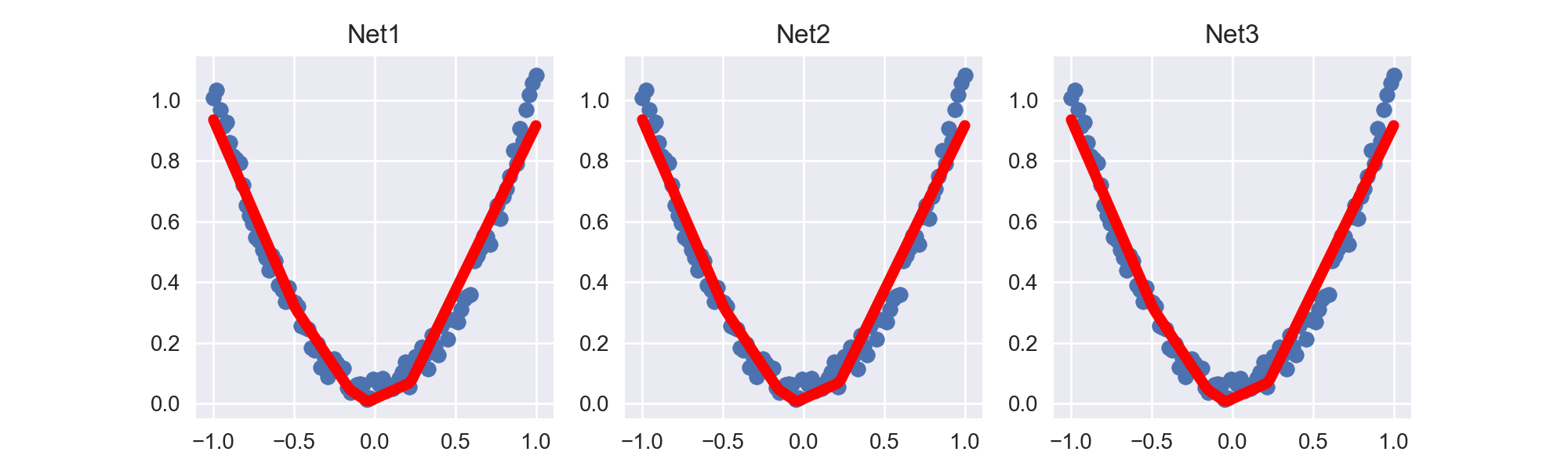
hidden layer nodes == 10
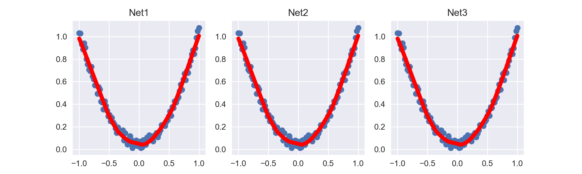
hidden layer nodes == 100, 增加宽度后拟合效果明显好与hidden layer nodes == 10的网络.
完整代码:
import os
os.environ['KMP_DUPLICATE_LIB_OK']='True'
import imageio
from tqdm import tqdm
import torch as t
import torch.nn as nn
import matplotlib.pyplot as plt
plt.style.use('seaborn') # 设置使用的样式
t.manual_seed(1) # reproducible
# 假数据
x = t.unsqueeze(t.linspace(-1, 1, 100), dim=1) # x data (tensor), shape=(100, 1)
y = x.pow(2) + 0.2*t.rand(x.size()) # noisy y data (tensor), shape=(100, 1)
def savemodel():
"""
保存网络
"""
# Build Net
net1 = nn.Sequential(
nn.Linear(1, 10),
nn.ReLU(),
nn.Linear(10, 1)
)
optimizer = t.optim.SGD(net1.parameters(), lr=0.5)
loss_func = t.nn.MSELoss()
# Train
for _ in range(100):
prediction = net1(x)
loss = loss_func(prediction, y)
optimizer.zero_grad()
loss.backward()
optimizer.step()
"""Save model"""
    t.save(net1, './Try_ModelSaved/net.pkl')  # 保存整个网络
    t.save(net1.state_dict(), './Try_ModelSaved/net_params.pkl')  # 只保存参数,速度快
def restore_net():
"""
提取整个网络
网络大时可能会慢
"""
    net2 = t.load('./Try_ModelSaved/net.pkl')  # restore entire net1 to net2
    prediction = net2(x)
def restore_params():
"""
提取网络参数
提取参数, 放入新建的网络中
"""
    """新建 net3"""
    net3 = t.nn.Sequential(
        nn.Linear(1, 10),
        nn.ReLU(),
        nn.Linear(10, 1)
    )
    """将参数复制到net3中"""
    net3.load_state_dict(t.load('./Try_ModelSaved/net_params.pkl'))
    prediction = net3(x)
savemodel()
restore_net()
restore_params()DataLoader 是 torch 给你用来包装你的数据的工具.
DataLoader核心代码
细节:
step里数据不够一个batch_size时, 最后一个step会输出剩下的数据完整示例代码:
import os
os.environ['KMP_DUPLICATE_LIB_OK']='True'
import imageio
from tqdm import tqdm
import torch as t
import torch.nn as nn
import torch.utils.data as Data
import matplotlib.pyplot as plt
plt.style.use('seaborn')  # 设置使用的样式

t.manual_seed(1)    # reproducible

BATCH_SIZE = 5      # 批训练的数据个数

x = t.linspace(1, 10, 10)       # x data (torch tensor)
y = t.linspace(10, 1, 10)       # y data (torch tensor)

# 先转换成 torch 能识别的 Dataset
torch_dataset = Data.TensorDataset(x, y)

# 把 dataset 放入 DataLoader
loader = Data.DataLoader(
    dataset=torch_dataset,      # torch TensorDataset format
    batch_size=BATCH_SIZE,      # mini batch size
    shuffle=True,               # 要不要打乱数据 (打乱比较好)
    num_workers=2,              # 多线程来读数据
)

for epoch in range(3):
    for step, (batch_x, batch_y) in enumerate(loader):
        # 假设这里就是你训练的地方...

        # 打出来一些数据
        print('Epoch:', epoch, '| Step:', step, '| batch x:',
              batch_x.numpy(), '| batch y:', batch_y.numpy())
输出:
Epoch: 0 | Step: 0 | batch x: [ 5.  7. 10.  3.  4.] | batch y: [6. 4. 1. 8. 7.]
Epoch: 0 | Step: 1 | batch x: [2. 1. 8. 9. 6.] | batch y: [ 9. 10.  3.  2.  5.]
Epoch: 1 | Step: 0 | batch x: [ 4.  6.  7. 10.  8.] | batch y: [7. 5. 4. 1. 3.]
Epoch: 1 | Step: 1 | batch x: [5. 3. 2. 1. 9.] | batch y: [ 6.  8.  9. 10.  2.]
Epoch: 2 | Step: 0 | batch x: [ 4.  2.  5.  6. 10.] | batch y: [7. 9. 6. 5. 1.]
Epoch: 2 | Step: 1 | batch x: [3. 9. 1. 8. 7.] | batch y: [ 8. 2. 10. 3. 4.]主要有以下几种模式
图示:
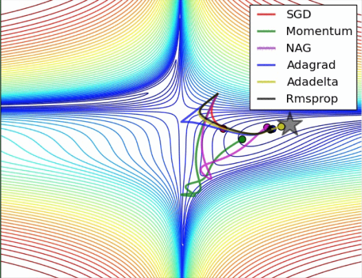
原始形式:

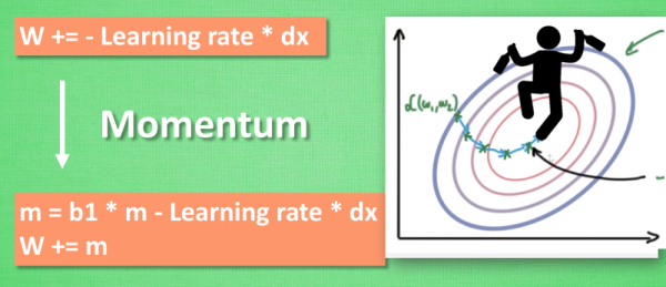
Momentum:
Adam:
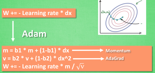
SGD是最普通的优化器, 也可以说没有加速效果, 而Momentum是SGD的改良版, 它加入了动量原则. 后面的RMSprop又是Momentum的升级版. 而Adam又是RMSprop的升级版. 不过从这个结果中我们看到,Adam的效果似乎比RMSprop要差一点. 所以说并不是越先进的优化器, 结果越佳. 我们在自己的试验中可以尝试不同的优化器, 找到那个最适合你数据/网络的优化器.
注意画不同的图的时候要建立不同的plt.figure()
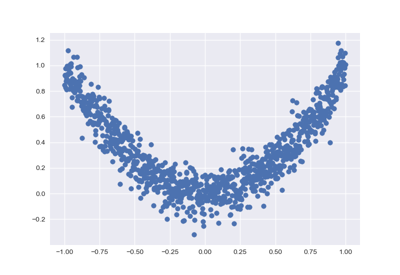
待分类数据:
 不同优化器对比结果:
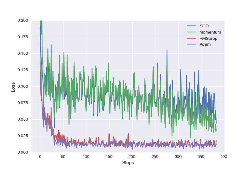
完整代码:
import os
os.environ['KMP_DUPLICATE_LIB_OK']='True'
import imageio
from tqdm import tqdm
import torch as t
import torch.nn as nn
import torch.utils.data as Data
import matplotlib.pyplot as plt
import torch.nn.functional as F
plt.style.use('seaborn')  # 设置使用的样式

t.manual_seed(1)    # reproducible

LR = 0.01
BATCH_SIZE = 32      # 批训练的数据个数
EPOCH = 12

# fake dataset
x = t.unsqueeze(t.linspace(-1, 1, 1000), dim=1)
y = x.pow(2) + 0.1*t.normal(t.zeros(*x.size()))

# 注意画不同的图的时候要建立不同的`plt.figure()`
plt.figure()
plt.scatter(x.numpy(), y.numpy())
plt.show()

# 使用上节内容提到的 data loader
torch_dataset = Data.TensorDataset(x, y)
loader = Data.DataLoader(dataset=torch_dataset, batch_size=BATCH_SIZE, shuffle=True, num_workers=2,)


# 为了对比每一种优化器, 我们给他们各自创建一个神经网络, 但这个神经网络都来自同一个 Net 形式.
class Net(nn.Module):
    def __init__(self):
        super(Net, self).__init__()
        self.hidden = nn.Linear(1, 10)
        self.predict = nn.Linear(10, 1)

    def forward(self, x):
        x = self.hidden(x)
        x = F.relu(x)
        x = self.predict(x)
        return x

net_SGD         = Net()
net_Momentum    = Net()
net_RMSprop     = Net()
net_Adam        = Net()
nets = [net_SGD, net_Momentum, net_RMSprop, net_Adam]

opt_SGD         = t.optim.SGD(net_SGD.parameters(), lr=LR)
opt_Momentum    = t.optim.SGD(net_Momentum.parameters(), lr=LR, momentum=0.8)
opt_RMSprop     = t.optim.RMSprop(net_RMSprop.parameters(), lr=LR, alpha=0.9)
opt_Adam        = t.optim.Adam(net_Adam.parameters(), lr=LR, betas=(0.9, 0.99))
optimizers = [opt_SGD, opt_Momentum, opt_RMSprop, opt_Adam]

loss_func = nn.MSELoss()
losses_his = [[], [], [], []]   # record the loss of 4 net

for epoch in range(EPOCH):
    print('Epoch:', epoch)
    for step, (b_x, b_y) in enumerate(loader):

        # 通过数组的形式, 迭代4次
        for net, opt, l_his in zip(nets, optimizers, losses_his):
            output = net(b_x)
            loss = loss_func(output, b_y)

            opt.zero_grad()
            loss.backward()
            opt.step()      # 为每个节点重设梯度
            l_his.append(loss.data.numpy())

# 注意画不同的图的时候要建立不同的`plt.figure()`
plt.figure()
labels = ['SGD', 'Momentum', 'RMSprop', 'Adam']
for i, l_his in enumerate(losses_his):
    plt.plot(l_his, label=labels[i])
plt.legend(loc='best')
plt.xlabel('Steps')
plt.ylabel('Loss')
plt.ylim((0, 0.2))
plt.show()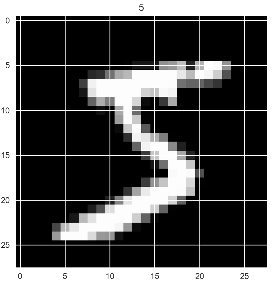
下载数据集方法
t-SNE聚类及可视化
low_dim_embs = tsne.fit_transform(last_layer.data.numpy()[:plot_only, :]), ==通过最后一层的pixel进行t-SNE分类可视化==
CNN模型
class CNN(t.nn.Module):
def __init__(self):
super(CNN, self).__init__()
self.conv1 = nn.Sequential(
# input shape (1, 28, 28) -> (16, 28, 28) -> (16, 14, 14)
nn.Conv2d(in_channels=1, out_channels=16, kernel_size=5, stride=1, padding=2), # conv后的图片大小不变
nn.ReLU(),
nn.MaxPool2d(kernel_size=2))
self.conv2 = nn.Sequential(
# input shape (16, 14, 14) -> (32, 14, 14) -> (32, 7, 7)
nn.Conv2d(in_channels=16, out_channels=32, kernel_size=5, stride=1, padding=2),
nn.ReLU(),
nn.MaxPool2d(kernel_size=2))
self.out = nn.Linear(32 * 7 * 7, 10) # 注意:(32*7*7, 10)
def forward(self, x):
x = self.conv1(x)
x = self.conv2(x)
x = x.view(x.size(0), -1) # 注意要将输入展开成一维向量(batch_size, 32*7*7)
output = self.out(x)
return output, x # 一定注意: 可视化时 return x for visualization CNN结构输出:
CNN(
(conv1): Sequential(
(0): Conv2d(1, 16, kernel_size=(5, 5), stride=(1, 1), padding=(2, 2))
(1): ReLU()
(2): MaxPool2d(kernel_size=2, stride=2, padding=0, dilation=1, ceil_mode=False)
)
(conv2): Sequential(
(0): Conv2d(16, 32, kernel_size=(5, 5), stride=(1, 1), padding=(2, 2))
(1): ReLU()
(2): MaxPool2d(kernel_size=2, stride=2, padding=0, dilation=1, ceil_mode=False)
)
(out): Linear(in_features=1568, out_features=10, bias=True)
)测试集前10个样本输出预测
[7 2 1 0 4 1 4 9 5 9] prediction number
[7 2 1 0 4 1 4 9 5 9] real number完整代码:
import os
os.environ['KMP_DUPLICATE_LIB_OK'] = 'True'
import imageio
from tqdm import tqdm
import torch as t
import torch.nn as nn
import torch.utils.data as Data
import matplotlib.pyplot as plt
import torch.nn.functional as F
import torchvision
plt.style.use('seaborn') # 设置使用的样式
# for visualization
from matplotlib import cm
try:
from sklearn.manifold import TSNE; HAS_SK = True
except:
HAS_SK = False; print('Please install sklearn for layer visualization')
LR = 0.001
BATCH_SIZE = 50 # 批训练的数据个数
EPOCH = 8
DOWNLOAD_MNIST = False
"""Mnist digits dataset"""
if not(os.path.exists('Volumes/ArcFile/mnist/')) or not os.listdir('Volumes/ArcFile/mnist/'):
DOWNLOAD_MNIST = True
train_data = torchvision.datasets.MNIST(
    root='Volumes/ArcFile/mnist/',
    train=True,  # this is training data
    # PIL.Image or numpy.ndarray to torch.FloatTensor(C * H * W), and normalize in the range [0.0, 1.0]
    transform=torchvision.transforms.ToTensor(),

    download=DOWNLOAD_MNIST
)
# 批训练 50samples, 1 channel, 28x28 (50, 1, 28, 28)
train_loader = Data.DataLoader(dataset=train_data, batch_size=BATCH_SIZE, shuffle=True)
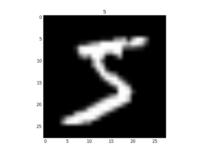
# plot one example
print(train_data.train_data.size()) # (60000, 28, 28)
print(train_data.train_labels.size()) # (60000)
plt.imshow(train_data.train_data[0].numpy(), cmap='gray')
plt.title('%i' % train_data.train_labels[0])
plt.show()
# pick 2000 samples to speed up testing
test_data = torchvision.datasets.MNIST(root='Volumes/ArcFile/mnist/', train=False)
# shape from (2000, 28, 28) to (2000, 1, 28, 28), value in range(0,1)
test_x = t.unsqueeze(test_data.test_data, dim=1).type(t.FloatTensor)[:2000] / 255.
test_y = test_data.test_labels[:2000]
class CNN(t.nn.Module):
    def __init__(self):
        super(CNN, self).__init__()
        self.conv1 = nn.Sequential(
            # input shape (1, 28, 28) -> (16, 28, 28) -> (16, 14, 14)
            nn.Conv2d(in_channels=1, out_channels=16, kernel_size=5, stride=1, padding=2),  # conv后的图片大小不变
            nn.ReLU(),
            nn.MaxPool2d(kernel_size=2))
        self.conv2 = nn.Sequential(
            # input shape (16, 14, 14) -> (32, 14, 14) -> (32, 7, 7)
            nn.Conv2d(in_channels=16, out_channels=32, kernel_size=5, stride=1, padding=2),
            nn.ReLU(),
            nn.MaxPool2d(kernel_size=2))
        self.out = nn.Linear(32 * 7 * 7, 10)  # 注意:(32*7*7, 10)

    def forward(self, x):
        x = self.conv1(x)
        x = self.conv2(x)
        x = x.view(x.size(0), -1)  # 注意要将输入展开成一维向量(batch_size, 32*7*7)
        output = self.out(x)
        return output, x        # 一定注意: 可视化时 return x for visualization
cnn = CNN()
print(cnn)
optimizer = t.optim.Adam(cnn.parameters(), lr=LR, betas=(0.9, 0.99))
loss_func = nn.CrossEntropyLoss()
def plot_with_labels(lowDWeights, labels, image_list, *param):
plt.cla()
X, Y = lowDWeights[:, 0], lowDWeights[:, 1]
epoch, loss, accuracy = param
for x, y, s in zip(X, Y, labels):
c = cm.rainbow(int(255 * s / 9))
plt.text(x, y, s, backgroundcolor=c, fontsize=9)
# plt.xlim(X.min(), X.max())
# plt.ylim(Y.min(), Y.max())
plt.xlim(-50, 50)
plt.ylim(-40, 40)
plt.title('Visualize last layer')
text = ('Epoch: %d,' % epoch + ' train loss: %.4f,' % loss.data.numpy() + ' test accuracy: %.3f' % accuracy)
plt.text(-30, -35, text, fontdict={'size': 13, 'color': 'red'})
plt.show()
plt.savefig("temp.jpg")
plt.pause(0.02)
image_list.append(imageio.imread("temp.jpg")) # 可以不用循环i,直接用列表形式
def Train():
plt.ion()
image_list = []
for epoch in tqdm(range(EPOCH)):
for step, (b_x, b_y) in enumerate(train_loader):
output = cnn(b_x)[0] # 注意如果需要visualization时会有2个返回值,故要选择
loss = loss_func(output, b_y)
optimizer.zero_grad() # 计算完损失就可以清除梯度了
loss.backward()
optimizer.step()
# visualization use t-SNE
if step % 100 == 0:
test_output, last_layer = cnn(test_x)
pred_y = t.max(test_output, 1)[1].data.numpy()
accuracy = float((pred_y == test_y.data.numpy()).astype(int).sum()) / float(test_y.size(0))
print('Epoch: ', epoch, '| train loss: %.4f' % loss.data.numpy(), '| test accuracy: %.3f' % accuracy)
if HAS_SK:
# Visualization of trained flatten layer (T-SNE)
tsne = TSNE(perplexity=30, n_components=2, init='pca', n_iter=5000)
plot_only = 500
low_dim_embs = tsne.fit_transform(last_layer.data.numpy()[:plot_only, :])
labels = test_y.numpy()[:plot_only]
plot_with_labels(low_dim_embs, labels, image_list, epoch, loss, accuracy) # lowDWeights, labels
plt.ioff()
imageio.mimsave('CNN_MNIST.gif', image_list, 'GIF', duration=0.2)
t.save(cnn, './Try_ModelSaved/cnn_mnist.pkl') # 保存整个网络
def Test():
net2 = t.load('./Try_ModelSaved/cnn_mnist.pkl') # restore entire net1 to net2
test_output = net2(test_x[:10])
pred_y = t.max(test_output[0], 1)[1].data.numpy().squeeze()
print(pred_y, 'prediction number')
print(test_y[:10].numpy(), 'real number')
Train()
Test()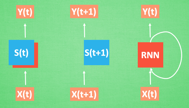
梯度消失或者梯度爆炸的问题(取决于w大于1还是小于1)
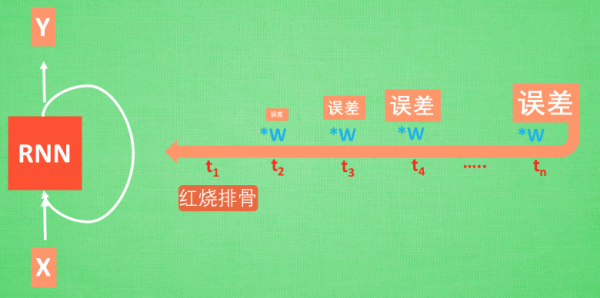
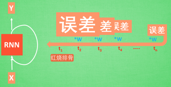
带控制器 — 输入控制,输出控制,忘记控制

RNN模型: 和以前一样, 我们用一个 class 来建立 RNN 模型. 这个 RNN 整体流程是
(input0, state0) -> LSTM -> (output0, state1);(input1, state1) -> LSTM -> (output1, state2);(inputN, stateN)-> LSTM -> (outputN, stateN+1);outputN -> Linear -> prediction. 通过LSTM分析每一时刻的值, 并且将这一时刻和前面时刻的理解合并在一起, 生成当前时刻对前面数据的理解或记忆. 传递这种理解给下一时刻分析.
输出:
torch.Size([60000, 28, 28])
torch.Size([60000])
RNN(
(rnn): LSTM(28, 64, batch_first=True)
(out): Linear(in_features=64, out_features=10, bias=True)
)
Epoch: 0 | train loss: 2.2925 | test accuracy: 0.10
Epoch: 0 | train loss: 1.1347 | test accuracy: 0.55
Epoch: 0 | train loss: 1.0238 | test accuracy: 0.68
Epoch: 0 | train loss: 0.4887 | test accuracy: 0.81
Epoch: 0 | train loss: 0.4760 | test accuracy: 0.85
Epoch: 0 | train loss: 0.2999 | test accuracy: 0.86
Epoch: 0 | train loss: 0.3342 | test accuracy: 0.89
Epoch: 0 | train loss: 0.4210 | test accuracy: 0.93
Epoch: 0 | train loss: 0.1264 | test accuracy: 0.93
Epoch: 0 | train loss: 0.3789 | test accuracy: 0.93
Epoch: 0 | train loss: 0.2171 | test accuracy: 0.92
Epoch: 0 | train loss: 0.2132 | test accuracy: 0.94
Epoch: 0 | train loss: 0.2326 | test accuracy: 0.93
Epoch: 0 | train loss: 0.0600 | test accuracy: 0.94
Epoch: 0 | train loss: 0.2595 | test accuracy: 0.94
Epoch: 0 | train loss: 0.0987 | test accuracy: 0.95
Epoch: 0 | train loss: 0.1818 | test accuracy: 0.94
Epoch: 0 | train loss: 0.3106 | test accuracy: 0.96
Epoch: 0 | train loss: 0.1822 | test accuracy: 0.95
[7 2 1 0 4 1 4 9 5 9] prediction number
[7 2 1 0 4 1 4 9 5 9] real number完整程序:
import os
os.environ['KMP_DUPLICATE_LIB_OK'] = 'True'
import imageio
from tqdm import tqdm
import torch as t
import torch.nn as nn
import torch.utils.data as Data
import matplotlib.pyplot as plt
import torch.nn.functional as F
import torchvision
import torchvision.transforms as transforms
plt.style.use('seaborn') # 设置使用的样式
# for visualization
from matplotlib import cm
try:
from sklearn.manifold import TSNE; HAS_SK = True
except:
HAS_SK = False; print('Please install sklearn for layer visualization')
LR = 0.01
BATCH_SIZE = 64
EPOCH = 1
TIME_STEP = 28      # rnn 时间步数 / 图片高度
INPUT_SIZE = 28     # rnn 每步输入值 / 图片每行像素
DOWNLOAD_MNIST = False
"""Mnist digits dataset"""
if not(os.path.exists('/Volumes/ArcFile/mnist/')) or not os.listdir('/Volumes/ArcFile/mnist/'):
DOWNLOAD_MNIST = True
train_data = torchvision.datasets.MNIST(
root='/Volumes/ArcFile/mnist/',
train=True, # this is training data
# PIL.Image or numpy.ndarray to torch.FloatTensor(C * H * W), and normalize in the range [0.0, 1.0]
transform=transforms.ToTensor(),
download=DOWNLOAD_MNIST
)
# 批训练 50samples, 1 channel, 28x28 (50, 1, 28, 28)
train_loader = Data.DataLoader(dataset=train_data, batch_size=BATCH_SIZE, shuffle=True)
# plot one example
print(train_data.train_data.size()) # (60000, 28, 28)
print(train_data.train_labels.size()) # (60000)
plt.imshow(train_data.train_data[0].numpy(), cmap='gray')
plt.title('%i' % train_data.train_labels[0])
plt.show()
# pick 2000 samples to speed up testing
test_data = torchvision.datasets.MNIST(root='/Volumes/ArcFile/mnist/', train=False, transform=transforms.ToTensor())
# shape from (2000, 28, 28) to (2000, 1, 28, 28), value in range(0,1)
test_x = test_data.test_data.type(t.FloatTensor)[:2000] / 255. # 注意这里不需要unsqueeze()数据了,因为RNN只需要3个??
test_y = test_data.test_labels.numpy()[:2000]
class RNN(t.nn.Module):
def __init__(self):
super(RNN, self).__init__()
self.rnn = nn.LSTM( # LSTM 效果要比 nn.RNN() 好多了
input_size=28, # 图片每行的数据像素点
hidden_size=64, # rnn hidden unit
num_layers=1, # 有几层 RNN layers
batch_first=True, # input & output 会是以 batch size 为第一维度的特征集 e.g. (batch, time_step, input_size)
)
self.out = nn.Linear(64, 10) # 输出层
def forward(self, x):
# x shape (batch, time_step, input_size)
# r_out shape (batch, time_step, output_size)
# h_n shape (n_layers, batch, hidden_size) LSTM 有两个 hidden states, h_n 是分线, h_c 是主线
# h_c shape (n_layers, batch, hidden_size)
r_out, (h_n, h_c) = self.rnn(x, None) # None 表示 hidden state 会用全0的 state
# 选取最后一个时间点的 r_out 输出
# 这里 r_out[:, -1, :] 的值也是 h_n 的值
out = self.out(r_out[:, -1, :])
return out
rnn = RNN()
print(rnn)
"""
RNN (
(rnn): LSTM(28, 64, batch_first=True)
(out): Linear (64 -> 10)
)
"""
optimizer = t.optim.Adam(rnn.parameters())
loss_func = nn.CrossEntropyLoss()
def plot_with_labels(lowDWeights, labels, image_list, *param):
plt.cla()
X, Y = lowDWeights[:, 0], lowDWeights[:, 1]
epoch, loss, accuracy = param
for x, y, s in zip(X, Y, labels):
c = cm.rainbow(int(255 * s / 9))
plt.text(x, y, s, backgroundcolor=c, fontsize=9)
# plt.xlim(X.min(), X.max())
# plt.ylim(Y.min(), Y.max())
plt.xlim(-50, 50)
plt.ylim(-40, 40)
plt.title('Visualize last layer')
text = ('Epoch: %d,' % epoch + ' train loss: %.4f,' % loss.data.numpy() + ' test accuracy: %.3f' % accuracy)
plt.text(-30, -35, text, fontdict={'size': 13, 'color': 'red'})
plt.show()
plt.savefig("temp.jpg")
plt.pause(0.02)
image_list.append(imageio.imread("temp.jpg")) # 可以不用循环i,直接用列表形式
def Train():
plt.ion()
# plt.figure(figsize=(5,5))
# image_list = []
for epoch in tqdm(range(EPOCH)):
for step, (b_x, b_y) in enumerate(train_loader):
b_x = b_x.view(-1, 28, 28) # reshape x to (batch, time_step, input_size)
output = rnn(b_x) # 注意如果需要visualization时会有2个返回值,故要选择
loss = loss_func(output, b_y)
optimizer.zero_grad() # 计算完损失就可以清除梯度了
loss.backward()
optimizer.step()
# visualization use t-SNE
if step % 100 == 0:
test_output = rnn(test_x) # x 赋值给 last_layer
pred_y = t.max(test_output, 1)[1].data.numpy()
accuracy = float((pred_y == test_y).astype(int).sum()) / float(test_y.size)
print('Epoch: ', epoch, '| train loss: %.4f' % loss.data.numpy(), '| test accuracy: %.3f' % accuracy)
# if HAS_SK:
# # Visualization of trained flatten layer (T-SNE)
# tsne = TSNE(perplexity=30, n_components=2, init='pca', n_iter=5000)
# plot_only = 500
# low_dim_embs = tsne.fit_transform(last_layer.data.numpy()[:plot_only, :]) # 通过最后一层的pixel进行t-SNE分类可视化
# labels = test_y.numpy()[:plot_only]
# plot_with_labels(low_dim_embs, labels, image_list, epoch, loss, accuracy) # lowDWeights, labels
# plt.ioff()
# imageio.mimsave('RNN_MNIST.gif', image_list, 'GIF', duration=0.2)
t.save(rnn, './Try_ModelSaved/rnn_mnist.pkl') # 保存整个网络
def Test():
net2 = t.load('./Try_ModelSaved/rnn_mnist.pkl') # restore entire net1 to net2
test_output = net2(test_x[:10])
pred_y = t.max(test_output, 1)[1].data.numpy().squeeze()
print(pred_y, 'prediction number')
print(test_y[:10], 'real number')
Train()
Test()
import torch
from torch import nn
import torchvision.datasets as dsets
import torchvision.transforms as transforms
import matplotlib.pyplot as plt
# torch.manual_seed(1) # reproducible
# Hyper Parameters
EPOCH = 1 # train the training data n times, to save time, we just train 1 epoch
BATCH_SIZE = 64
TIME_STEP = 28 # rnn time step / image height
INPUT_SIZE = 28 # rnn input size / image width
LR = 0.01 # learning rate
DOWNLOAD_MNIST = True # set to True if haven't download the data
# Mnist digital dataset
train_data = dsets.MNIST(
root='./mnist/',
train=True, # this is training data
transform=transforms.ToTensor(), # Converts a PIL.Image or numpy.ndarray to
# torch.FloatTensor of shape (C x H x W) and normalize in the range [0.0, 1.0]
download=DOWNLOAD_MNIST, # download it if you don't have it
)
# plot one example
print(train_data.train_data.size()) # (60000, 28, 28)
print(train_data.train_labels.size()) # (60000)
plt.imshow(train_data.train_data[0].numpy(), cmap='gray')
plt.title('%i' % train_data.train_labels[0])
plt.show()
# Data Loader for easy mini-batch return in training
train_loader = torch.utils.data.DataLoader(dataset=train_data, batch_size=BATCH_SIZE, shuffle=True)
# convert test data into Variable, pick 2000 samples to speed up testing
test_data = dsets.MNIST(root='./mnist/', train=False, transform=transforms.ToTensor())
test_x = test_data.test_data.type(torch.FloatTensor)[:2000]/255. # shape (2000, 28, 28) value in range(0,1)
test_y = test_data.test_labels.numpy()[:2000] # covert to numpy array
class RNN(nn.Module):
def __init__(self):
super(RNN, self).__init__()
self.rnn = nn.LSTM( # if use nn.RNN(), it hardly learns
input_size=INPUT_SIZE,
hidden_size=64, # rnn hidden unit
num_layers=1, # number of rnn layer
batch_first=True, # input & output will has batch size as 1s dimension. e.g. (batch, time_step, input_size)
)
self.out = nn.Linear(64, 10)
def forward(self, x):
# x shape (batch, time_step, input_size)
# r_out shape (batch, time_step, output_size)
# h_n shape (n_layers, batch, hidden_size)
# h_c shape (n_layers, batch, hidden_size)
r_out, (h_n, h_c) = self.rnn(x, None) # None represents zero initial hidden state
# choose r_out at the last time step
out = self.out(r_out[:, -1, :])
return out
rnn = RNN()
print(rnn)
optimizer = torch.optim.Adam(rnn.parameters(), lr=LR) # optimize all cnn parameters
loss_func = nn.CrossEntropyLoss() # the target label is not one-hotted
# training and testing
for epoch in range(EPOCH):
for step, (b_x, b_y) in enumerate(train_loader): # gives batch data
b_x = b_x.view(-1, 28, 28) # reshape x to (batch, time_step, input_size)
output = rnn(b_x) # rnn output
loss = loss_func(output, b_y) # cross entropy loss
optimizer.zero_grad() # clear gradients for this training step
loss.backward() # backpropagation, compute gradients
optimizer.step() # apply gradients
if step % 50 == 0:
test_output = rnn(test_x) # (samples, time_step, input_size)
pred_y = torch.max(test_output, 1)[1].data.numpy()
accuracy = float((pred_y == test_y).astype(int).sum()) / float(test_y.size)
print('Epoch: ', epoch, '| train loss: %.4f' % loss.data.numpy(), '| test accuracy: %.2f' % accuracy)
# print 10 predictions from test data
test_output = rnn(test_x[:10].view(-1, 28, 28))
pred_y = torch.max(test_output, 1)[1].data.numpy()
print(pred_y, 'prediction number')
print(test_y[:10], 'real number')
前向传播过程
def forward(self, x, h_state):
    # 因为 hidden state 是连续的, 所以我们要一直传递这一个 state
    # x (batch, time_step, input_size)
    # h_state (n_layers, batch, hidden_size)
    # r_out (batch, time_step, output_size)
    # h_state是之前事情的记忆, 也要作为 RNN 的一个输入
    r_out, h_state = self.rnn(x, h_state)

    outs = []    # 保存所有时间点的预测值, 利用动态图
    for time_step in range(r_out.size(1)):    # 对每一个时间点计算 output
        outs.append(self.out(r_out[:, time_step, :]))  # 每个time_step计算
    return t.stack(outs, dim=1), h_state    # t.stack(): list -> tensor
预测过程
完整代码:
import os
os.environ['KMP_DUPLICATE_LIB_OK'] = 'True'
import imageio
from tqdm import tqdm
import torch as t
import torch.nn as nn
import torch.utils.data as Data
import matplotlib.pyplot as plt
import torch.nn.functional as F
import torchvision
import torchvision.transforms as transforms
import numpy as np
plt.style.use('seaborn')
LR = 0.02
BATCH_SIZE = 64
TIME_STEP = 10 # rnn 时间步数 / 图片高度
INPUT_SIZE = 1 # rnn 每步输入值 / 图片每行像素
# show data
steps = np.linspace(0, np.pi * 2, 100, dtype=np.float32) # float32 for converting torch FloatTensor
x_np = np.sin(steps)
y_np = np.cos(steps)
plt.plot(steps, y_np, 'r-', label='target (cos)')
plt.plot(steps, x_np, 'b-', label='input (sin)')
plt.legend(loc='best')
plt.show()
class RNN(t.nn.Module):
def __init__(self):
super(RNN, self).__init__()
self.rnn = nn.RNN( # 注意这里是RNN就够了
input_size=INPUT_SIZE, # 函数幅度是1
hidden_size=32, # rnn hidden unit
num_layers=1, # 有几层 RNN layers
batch_first=True, # input & output 会是以 batch size 为第一维度的特征集 e.g. (batch, time_step, input_size)
)
self.out = nn.Linear(32, 1) # 输出层
def forward(self, x, h_state):
# 因为 hidden state 是连续的, 所以我们要一直传递这一个 state
# x (batch, time_step, input_size)
# h_state (n_layers, batch, hidden_size)
# r_out (batch, time_step, output_size)
# h_state是之前事情的记忆, 也要作为 RNN 的一个输入
r_out, h_state = self.rnn(x, h_state)
outs = [] # 保存所有时间点的预测值, 利用动态图
for time_step in range(r_out.size(1)): # 对每一个时间点计算 output
outs.append(self.out(r_out[:, time_step, :])) # 每个time_step计算
return t.stack(outs, dim=1), h_state # t.stack(): list -> tensor
#
rnn = RNN()
print(rnn)
"""
RNN (
(rnn): RNN(1, 32, batch_first=True)
(out): Linear (32 -> 1)
)
"""
optimizer = t.optim.Adam(rnn.parameters(), lr=LR)
loss_func = nn.MSELoss()
def Train():
plt.ion()
h_state = None # for initial hidden state, 因为最初没有前面的数据
plt.figure(1, figsize=(12, 5))
image_list = []
for step in tqdm(range(100)):
start, end = step * np.pi, (step + 1) * np.pi # time steps, 截取一小段起始位置
# sin 预测 cos
steps = np.linspace(start, end, 10, dtype=np.float32, endpoint=False)
x_np = np.sin(steps) # float32 for converting torch FloatTensor
y_np = np.cos(steps)
x = t.from_numpy(x_np[np.newaxis, :, np.newaxis]) # shape (batch, time_step, input_size) 加1个维度
y = t.from_numpy(y_np[np.newaxis, :, np.newaxis])
    prediction, h_state = rnn(x, h_state)  # rnn 对于每个 step 的 prediction, 还有最后一个 step 的 h_state
    # !!  下一步十分重要 !! 否则无法反向传播
    h_state = h_state.data  # 要把 h_state 重新包装一下才能放入下一个 iteration, 不然会报错
loss = loss_func(prediction, y)
optimizer.zero_grad()
loss.backward()
optimizer.step()
plt.plot(steps, y_np.flatten(), 'r-')
plt.plot(steps, prediction.data.numpy().flatten(), 'b-')
plt.draw()
plt.savefig('temp.jpg')
plt.pause(0.05)
if step % 4 == 0:
image_list.append(imageio.imread('temp.jpg'))
imageio.mimsave('RNN_MNIST.gif', image_list, 'GIF', duration=0.2)
plt.ioff()
plt.show()
Train()自编码是一种神经网络的形式
对自编码器的训练, 相当于将图片经过了压缩,再解压的这一道工序. 当压缩的时候, 原有的图片质量被缩减, 解压时用信息量小却包含了所有关键信息的文件恢复出原本的图片.
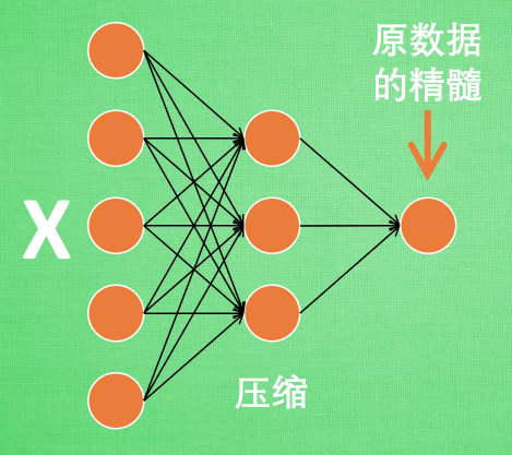
编码器: 进而可以训练编码器可以提取足够的有用信息以够恢复原始数据.实际使用时只使用前半部分, 目的是经过编码器网络可以极大减少数据量却不损失关键信息(提取关键特征)
==自编码器能自动分类数据, 也可以其那套在半监督上, 用少量有标签样本和大量无标签样本进行学习.==

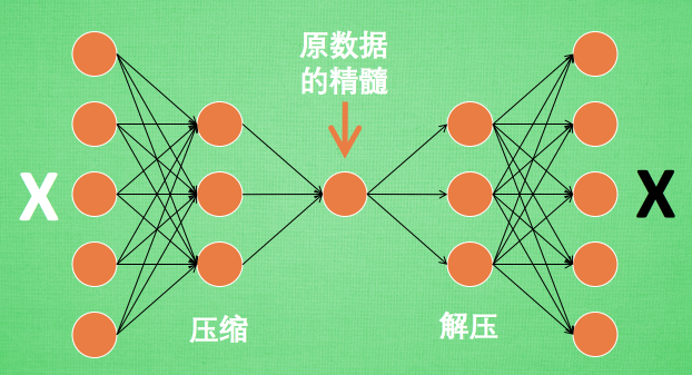
编码器能得到原数据的精髓, 然后我们只需要再创建一个小的神经网络学习这个精髓的数据,不仅减少了神经网络的负担, 而且同样能达到很好的效果.
自编码是类似于PCA可以对特征属性降维, 以用来区分原数据. 效果甚至超越PCA
解码器训练时是用来将精髓信息解压成原始信息, 所以可以认为是类似于解压器或者生成器的作用(类似GAN), 那做这件事的一种特殊自编码叫做 variational autoencoders,
VAE解释: Variational Autoencoders Explained
有一个例子就是让它能模仿并生成手写数字.
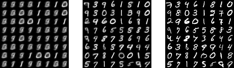
只需要使用training data, 且不需要labels
训练过程(上面是输入图片, 下面是网络选择的图片)
可以看出5和3,4和9比较难分辨
最终分类图 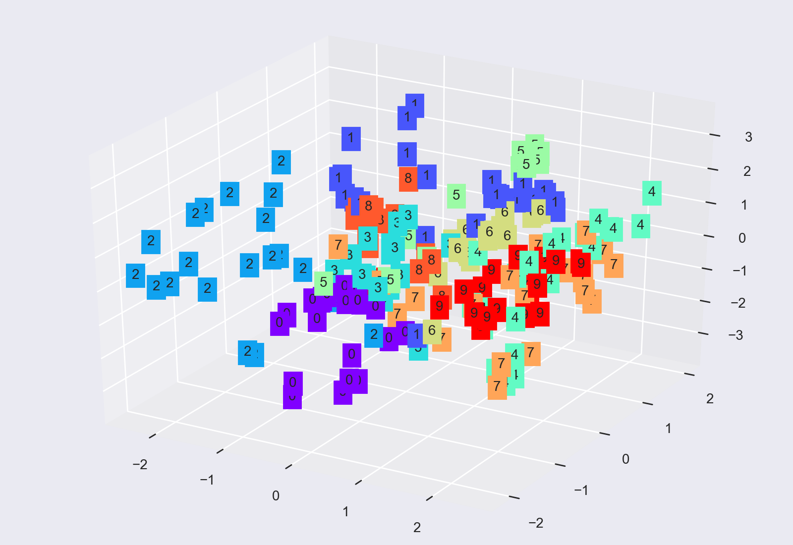
注意
class AutoEncoder(nn.Module):
    def __init__(self):
        super(AutoEncoder, self).__init__()
        # 压缩
        self.encoder = nn.Sequential(
            nn.Linear(28*28, 128),
            nn.Tanh(),
            nn.Linear(128, 64),
            nn.Tanh(),
            nn.Linear(64, 12),
            nn.Tanh(),
            nn.Linear(12, 3),   # 压缩成3个feature, 进行3D图像可视化
        )
        # 解压
        self.decoder = nn.Sequential(
            nn.Linear(3, 12),
            nn.Tanh(),
            nn.Linear(12, 64),
            nn.Tanh(),
            nn.Linear(64, 128),
            nn.Tanh(),
            nn.Linear(128, 28*28),
            nn.Sigmoid(),       # 激励函数是为了让输出值在 (0,1)
        )

    def forward(self, x):
        encoder = self.encoder(x)
        decoder = self.decoder(encoder)
        return encoder, decoder     # 注意要把encoder和decoder都输出
for epoch in range(EPOCH):
for step, (x, b_label) in tqdm(enumerate(train_loader)):
# 输出的目标图像是和输入完全相同的, 想要恢复的目标
b_x = x.view(-1, 28*28) # batch x, shape (batch, 28*28)
b_y = x.view(-1, 28*28) # batch y, shape (batch, 28*28)
encoder, decoder = autoencoder(b_x)
loss = loss_func(decoder, b_y) # 入图像向量和出图像向量差别为loss
optimizer.zero_grad() # 计算完损失就可以清除梯度了
loss.backward()
optimizer.step()完整代码:
import os
os.environ['KMP_DUPLICATE_LIB_OK'] = 'True'
import imageio
from tqdm import tqdm
import torch as t
import torch.nn as nn
import torch.utils.data as Data
import matplotlib.pyplot as plt
import torch.nn.functional as F
import torchvision
from mpl_toolkits.mplot3d import Axes3D
import numpy as np
import torchvision.transforms as transforms
plt.style.use('seaborn') # 设置使用的样式
# for visualization
from matplotlib import cm
from sklearn.manifold import TSNE; HAS_SK = True
LR = 0.005
BATCH_SIZE = 64 # 批训练的数据个数
EPOCH = 10
DOWNLOAD_MNIST = False
N_TEST_IMG = 5 # 到时候显示 5张图片看效果, 如上图一
"""Mnist digits dataset"""
if not(os.path.exists('/Volumes/ArcFile/mnist/')) or not os.listdir('/Volumes/ArcFile/mnist/'):
DOWNLOAD_MNIST = True
train_data = torchvision.datasets.MNIST(
root='/Volumes/ArcFile/mnist/',
train=True,
# PIL.Image or numpy.ndarray to torch.FloatTensor(C * H * W), and normalize in the range [0.0, 1.0]
transform=transforms.ToTensor(),
download=DOWNLOAD_MNIST
)
# Data Loader for easy mini-batch return in training, the image batch shape will be (50, 1, 28, 28)
train_loader = Data.DataLoader(dataset=train_data, batch_size=BATCH_SIZE, shuffle=True)
class AutoEncoder(nn.Module):
def __init__(self):
super(AutoEncoder, self).__init__()
# 压缩
self.encoder = nn.Sequential(
nn.Linear(28*28, 128),
nn.Tanh(),
nn.Linear(128, 64),
nn.Tanh(),
nn.Linear(64, 12),
nn.Tanh(),
nn.Linear(12, 3), # 压缩成3个feature, 进行3D图像可视化
)
# 解压
self.decoder = nn.Sequential(
nn.Linear(3, 12),
nn.Tanh(),
nn.Linear(12, 64),
nn.Tanh(),
nn.Linear(64, 128),
nn.Tanh(),
nn.Linear(128, 28*28),
nn.Sigmoid(), # 激励函数是为了让输出值在 (0,1)
)
def forward(self, x):
encoder = self.encoder(x)
decoder = self.decoder(encoder)
return encoder, decoder # 注意要把encoder和decoder都输出
autoencoder = AutoEncoder()
print(autoencoder)
optimizer = t.optim.Adam(autoencoder.parameters(), lr=LR)
loss_func = nn.MSELoss() # why??
def plot_with_labels(lowDWeights, labels, image_list, *param):
# 要观看的数据
view_data = train_data.train_data[:200].view(-1, 28 * 28).type(torch.FloatTensor) / 255.
encoded_data, _ = autoencoder(view_data) # 提取压缩的特征值
fig = plt.figure(2)
ax = Axes3D(fig) # 3D 图
# x, y, z 的数据值
X = encoded_data.data[:, 0].numpy()
Y = encoded_data.data[:, 1].numpy()
Z = encoded_data.data[:, 2].numpy()
values = train_data.train_labels[:200].numpy() # 标签值
for x, y, z, s in zip(X, Y, Z, values):
c = cm.rainbow(int(255 * s / 9)) # 上色
ax.text(x, y, z, s, backgroundcolor=c) # 标位子
ax.set_xlim(X.min(), X.max())
ax.set_ylim(Y.min(), Y.max())
ax.set_zlim(Z.min(), Z.max())
epoch, loss, accuracy = param
text = ('Epoch: %d,' % epoch + ' train loss: %.4f,' % loss.data.numpy() + ' test accuracy: %.3f' % accuracy)
plt.text(-30, -35, text, fontdict={'size': 13, 'color': 'red'})
plt.show()
plt.savefig("temp.jpg")
plt.pause(0.02)
image_list.append(imageio.imread("temp.jpg")) # 可以不用循环i,直接用列表形式
def Train():
# initialize figure
f, a = plt.subplots(2, N_TEST_IMG, figsize=(5, 2))
plt.ion() # continuously plot
# original data (first row) for viewing
view_data = train_data.train_data[:N_TEST_IMG].view(-1, 28 * 28).type(t.FloatTensor) / 255.
for i in range(N_TEST_IMG):
a[0][i].imshow(np.reshape(view_data.data.numpy()[i], (28, 28)), cmap='gray')
a[0][i].set_xticks(())
a[0][i].set_yticks(())
image_list = []
    for epoch in range(EPOCH):
        for step, (x, b_label) in tqdm(enumerate(train_loader)):
            # 输出的目标图像是和输入完全相同的, 想要恢复的目标
            b_x = x.view(-1, 28*28)  # batch x, shape (batch, 28*28)
            b_y = x.view(-1, 28*28)   # batch y, shape (batch, 28*28)

            encoder, decoder = autoencoder(b_x)

            loss = loss_func(decoder, b_y)  # 入图像向量和出图像向量差别为loss
            optimizer.zero_grad()  # 计算完损失就可以清除梯度了
            loss.backward()
            optimizer.step()
# visualization use t-SNE
if step % 50 == 0:
print('Epoch: ', epoch, '| train loss: %.4f' % loss.data.numpy())
# plotting decoded image (second row)
_, decoded_data = autoencoder(view_data)
for i in range(N_TEST_IMG):
a[1][i].clear()
a[1][i].imshow(np.reshape(decoded_data.data.numpy()[i], (28, 28)), cmap='gray')
a[1][i].set_xticks(())
a[1][i].set_yticks(())
plt.draw()
plt.savefig('temp.jpg')
plt.pause(0.05)
if step % 200 == 0:
image_list.append(imageio.imread('temp.jpg'))
plt.ioff()
imageio.mimsave('AE_MNIST.gif', image_list, 'GIF', duration=0.2)
t.save(autoencoder, './Try_ModelSaved/autoencoder_mnist.pkl') # 保存整个网络
Train()
# visualize in 3D plot
view_data = train_data.train_data[:200].view(-1, 28*28).type(t.FloatTensor)/255.
encoded_data, _ = autoencoder(view_data)
fig = plt.figure(2); ax = Axes3D(fig)
X, Y, Z = encoded_data.data[:, 0].numpy(), encoded_data.data[:, 1].numpy(), encoded_data.data[:, 2].numpy()
values = train_data.train_labels[:200].numpy()
for x, y, z, s in zip(X, Y, Z, values):
c = cm.rainbow(int(255*s/9)); ax.text(x, y, z, s, backgroundcolor=c)
ax.set_xlim(X.min(), X.max()); ax.set_ylim(Y.min(), Y.max()); ax.set_zlim(Z.min(), Z.max())
plt.show()RL中用表格村春每个状态state 和 在这个状态下每个行为action所拥有的Q值. 但当今问题太复杂, 状态非常多, 其存储和搜索都很难. 所以引入神经网络.
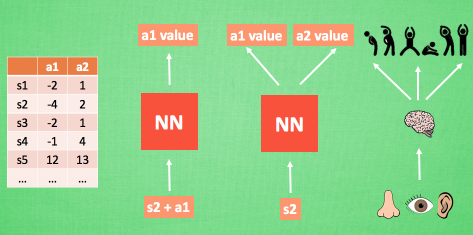
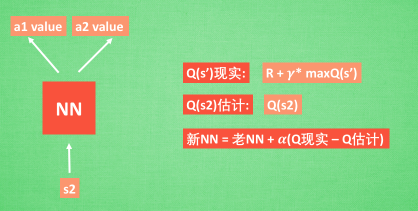
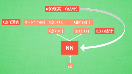
我们通过 NN 预测出Q(s2, a1) 和 Q(s2,a2) 的值, 这就是 Q 估计.
然后我们选取 Q 估计中最大值的动作来换取环境中的奖励 reward.
而 Q 现实中也包含从神经网络分析出来的两个 Q 估计值, 不过这个 Q 估计是针对于下一步在 s’ 的估计.
最后再通过算法更新神经网络中的参数
还有两大因素支撑着 DQN 使得它变得无比强大. 这两大因素就是 Experience replay 和 Fixed Q-targets.
Q learning 是一种 off-policy 离线学习法, 它能学习当前经历着的, 也能学习过去经历过的, 甚至是学习别人的经历. 所以每次 DQN 更新的时候, 我们都可以随机抽取一些之前的经历进行学习. 随机抽取这种做法打乱了经历之间的相关性, 也使得神经网络更新更有效率. Fixed Q-targets 也是一种打乱相关性的机理, 如果使用 fixed Q-targets, 我们就会在 DQN 中使用到两个结构相同但参数不同的神经网络, 预测 Q 估计 的神经网络具备最新的参数, 而预测 Q 现实 的神经网络使用的参数则是很久以前的. 有了这两种提升手段, DQN 才能在一些游戏中超越人类.

import torch
import torch.nn as nn
import torch.nn.functional as F
import numpy as np
import gym

# 超参数
BATCH_SIZE = 32
LR = 0.01
EPSILON = 0.9               # 最优选择动作百分比
GAMMA = 0.9                 # 奖励递减参数
TARGET_REPLACE_ITER = 100   # Q 现实网络的更新频率
MEMORY_CAPACITY = 2000      # 记忆库大小
env = gym.make('CartPole-v0')   # 立杆子游戏
env = env.unwrapped             # ??????
N_ACTIONS = env.action_space.n  # 杆子能做的动作
N_STATES = env.observation_space.shape[0]   # 杆子能获取的环境信息数


class Net(nn.Module):
    def __init__(self, ):
        super(Net, self).__init__()
        self.fc1 = nn.Linear(N_STATES, 10)
        self.fc1.weight.data.normal_(0, 0.1)   # initialization, 正态分布随机生成起始参数值
        self.out = nn.Linear(10, N_ACTIONS)     # 输出价值
        self.out.weight.data.normal_(0, 0.1)   # initialization

    def forward(self, x):
        x = self.fc1(x)
        x = F.relu(x)
        actions_value = self.out(x)
        return actions_value


class DQN(object):
    def __init__(self):
        # 建立 target net 和 eval net 还有 memory
        self.eval_net, self.target_net = Net(), Net()   # 相同的网络,参数延迟更新

        self.learn_step_counter = 0     # 用于 target 更新计时
        self.memory_counter = 0         # 记忆库记数
        self.memory = np.zeros((MEMORY_CAPACITY, N_STATES * 2 + 2))     # 初始化记忆库
        self.optimizer = torch.optim.Adam(self.eval_net.parameters(), lr=LR)    # torch 的优化器
        self.loss_func = nn.MSELoss()   # 误差公式

    def choose_action(self, x):
        # 根据环境观测值选择动作的机制
        x = torch.unsqueeze(torch.FloatTensor(x), 0)
        # 这里只输入一个 sample
        if np.random.uniform() < EPSILON:   # 选最优动作
            actions_value = self.eval_net.forward(x)
            action = torch.max(actions_value, 1)[1].data.numpy()[0]     # return the argmax
        else:   # 选随机动作
            action = np.random.randint(0, N_ACTIONS)
        return action

    def store_transition(self, s, a, r, s_):
        # 存储记忆
        transition = np.hstack((s, [a, r], s_))
        # 如果记忆库满了, 就覆盖老数据
        index = self.memory_counter % MEMORY_CAPACITY
        self.memory[index, :] = transition
        self.memory_counter += 1

    def learn(self):
        # target 网络更新
        # 学习记忆库中的记忆
        if self.learn_step_counter % TARGET_REPLACE_ITER == 0:
            self.target_net.load_state_dict(self.eval_net.state_dict())
        self.learn_step_counter += 1

        # 抽取记忆库中的批数据
        sample_index = np.random.choice(MEMORY_CAPACITY, BATCH_SIZE)
        b_memory = self.memory[sample_index, :]
        b_s = torch.FloatTensor(b_memory[:, :N_STATES])
        b_a = torch.LongTensor(b_memory[:, N_STATES:N_STATES + 1].astype(int))
        b_r = torch.FloatTensor(b_memory[:, N_STATES + 1:N_STATES + 2])
        b_s_ = torch.FloatTensor(b_memory[:, -N_STATES:])

        # 针对做过的动作b_a, 来选 q_eval 的值, (q_eval 原本有所有动作的值)
        q_eval = self.eval_net(b_s).gather(1, b_a)  # shape (batch, 1)
        q_next = self.target_net(b_s_).detach()  # q_next 不进行反向传递误差, 所以 detach
        q_target = b_r + GAMMA * q_next.max(1)[0]  # shape (batch, 1)
        loss = self.loss_func(q_eval, q_target)

        # 计算, 更新 eval net
        self.optimizer.zero_grad()
        loss.backward()
        self.optimizer.step()

dqn = DQN() # 定义 DQN 系统

for i_episode in range(400):
    s = env.reset()
    while True:
        env.render()    # 显示实验动画
        a = dqn.choose_action(s)    # 行为

        # 选动作, 得到环境反馈
        s_, r, done, info = env.step(a)     # 根据行为得到的反馈

        # 修改 reward, 使 DQN 快速学习
        x, x_dot, theta, theta_dot = s_
        r1 = (env.x_threshold - abs(x)) / env.x_threshold - 0.8
        r2 = (env.theta_threshold_radians - abs(theta)) / env.theta_threshold_radians - 0.5
        r = r1 + r2

        # 存记忆
        dqn.store_transition(s, a, r, s_)        # 状态 动作 奖励 下一个状态 存储

        if dqn.memory_counter > MEMORY_CAPACITY:
            dqn.learn() # 记忆库满了就进行学习

        if done:    # 如果回合结束, 进入下回合
            break

s = s_import torch
import torch.nn as nn
import numpy as np
import matplotlib.pyplot as plt
# torch.manual_seed(1) # reproducible
# np.random.seed(1)
# Hyper Parameters
BATCH_SIZE = 64
LR_G = 0.0001 # learning rate for generator
LR_D = 0.0001 # learning rate for discriminator
N_IDEAS = 5 # 灵感(random noise)的个数
ART_COMPONENTS = 15 # it could be total point G can draw in the canvas
PAINT_POINTS = np.vstack([np.linspace(-1, 1, ART_COMPONENTS) for _ in range(BATCH_SIZE)])
# show our beautiful painting range
# plt.plot(PAINT_POINTS[0], 2 * np.power(PAINT_POINTS[0], 2) + 1, c='#74BCFF', lw=3, label='upper bound')
# plt.plot(PAINT_POINTS[0], 1 * np.power(PAINT_POINTS[0], 2) + 0, c='#FF9359', lw=3, label='lower bound')
# plt.legend(loc='upper right')
# plt.show()
def artist_works(): # painting from the famous artist (real target)
a = np.random.uniform(1, 2, size=BATCH_SIZE)[:, np.newaxis]
paintings = a * np.power(PAINT_POINTS, 2) + (a - 1) # 15个x, a*x^2+a-1
paintings = torch.from_numpy(paintings).float() # 转化成torch 的形式
return paintings
G = nn.Sequential( # Generator
# N_IDEAS=5 -> ART_COMPONENTS=15
nn.Linear(N_IDEAS, 128), # random ideas (could from normal distribution)
nn.ReLU(),
nn.Linear(128, ART_COMPONENTS), # making a painting from these random ideas
)
D = nn.Sequential( # Discriminator
nn.Linear(ART_COMPONENTS, 128), # receive art work either from the famous artist or a newbie like G
nn.ReLU(),
nn.Linear(128, 1),
nn.Sigmoid(), # 转化为判断为真的概率 [0,1]
)
opt_D = torch.optim.Adam(D.parameters(), lr=LR_D)
opt_G = torch.optim.Adam(G.parameters(), lr=LR_G)
plt.ion() # something about continuous plotting
for step in range(10000):
artist_paintings = artist_works() # real painting from artist
G_ideas = torch.randn(BATCH_SIZE, N_IDEAS, requires_grad=True) # random ideas\n
G_paintings = G(G_ideas) # fake painting from G (random ideas)
prob_artist1 = D(G_paintings) # D try to reduce this prob
G_loss = torch.mean(torch.log(1. - prob_artist1))
opt_G.zero_grad()
G_loss.backward()
opt_G.step()
prob_artist0 = D(artist_paintings) # 真判真概率 D try to increase this prob
prob_artist1 = D(G_paintings.detach()) # 假判真概率 D try to reduce this prob
D_loss = - torch.mean(torch.log(prob_artist0) + torch.log(1. - prob_artist1))
opt_D.zero_grad()
D_loss.backward(retain_graph=True) # 保留计算图 reusing computational graph
opt_D.step()
if step % 50 == 0: # plotting
plt.cla()
plt.plot(PAINT_POINTS[0], G_paintings.data.numpy()[0], c='#4AD631', lw=3, label='Generated painting', )
plt.plot(PAINT_POINTS[0], 2 * np.power(PAINT_POINTS[0], 2) + 1, c='#74BCFF', lw=3, label='upper bound')
plt.plot(PAINT_POINTS[0], 1 * np.power(PAINT_POINTS[0], 2) + 0, c='#FF9359', lw=3, label='lower bound')
plt.text(-.5, 2.3, 'D accuracy=%.2f (0.5 for D to converge)' % prob_artist0.data.numpy().mean(),
fontdict={'size': 13})
plt.text(-.5, 2, 'D score= %.2f (-1.38 for G to converge)' % -D_loss.data.numpy(), fontdict={'size': 13})
plt.ylim((0, 3));
plt.legend(loc='upper right', fontsize=10);
plt.draw();
plt.pause(0.01)
plt.ioff()
plt.show()